PFlow: Box#3 – 2D Fluid Solver

This is a small exercise to test how well Particle Flow’s Box#3 performs as a pseudo visual scripting tool.

PFlow 2D Fluid Solver

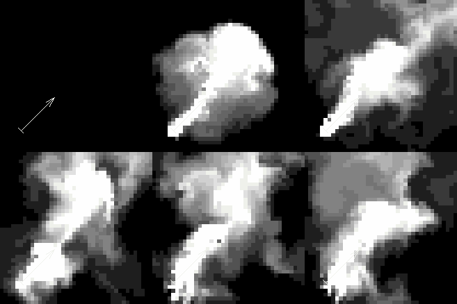
I chose a Java implementation of a 2D Fluid Solver from this website:
http://www.multires.caltech.edu/teaching/demos/java/stablefluids.htm
The above link has the Java code which I converted into MaxScript code for purposes of having a data medium to compare onto.

The Java code also implements Vorticity Confinement and Bouyancy Force for stabilizing velocities and simulating rising smoke – also implemented as Box#3 operators.

The solver is mostly based on the paper published by Jos Stam. With additional improvements from Ron Fedkiw and Henrik Jensen.
Real-Time Fluid Dynamics for Games by Jos Stam

---

Data Flow

Here is a screenshot of the Particle View:

Particle View

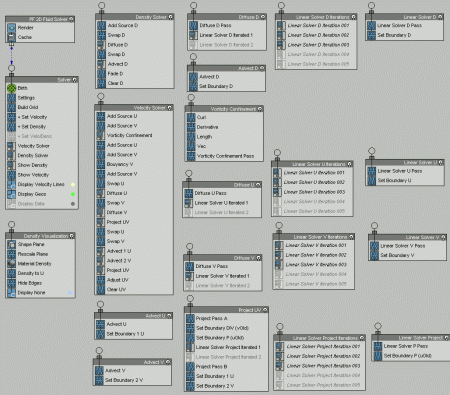
Notice here that Group Operators are used extensively. It enabled me to create blocks of Operators, similar to how blocks of codes are handled in MaxScript (or any other coding language). This greatly helped in organizing the flow and making sense of what each part would do.

Here is the same screenshot with added arrows to show the flow of data:

Particle View – Flow of Data

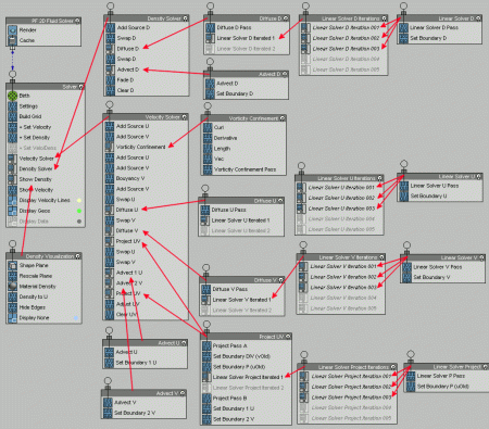
This also became essential to the solver, especially on parts where the code needed to have iterations.
Shown below is a sample concept of where a Group Operator allowed me to emulate an Iteration.

Iteration Example

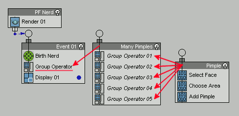
In the case above, the Pimple Event gets iterated 5 times inside the Many Pimples Event, so PF Nerd gets 5 pimple particles 🙂

---

Main Simulation Parameters

Here is a screenshot of the controls that I chose to expose. It is all shown by the Settings Operator.

Solver Settings

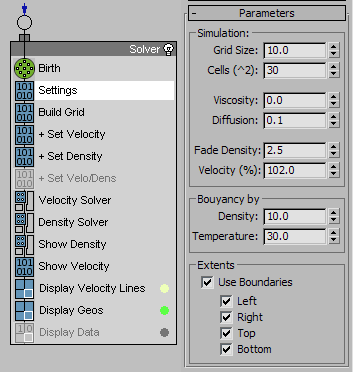
Grid Size – Size of the grid in world units.
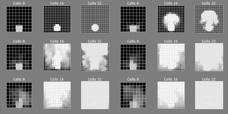
Cells (^2): Number of cells along the length and width of the Grid.
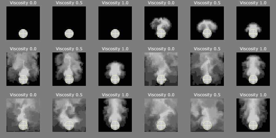
Viscosity: Counters the diffusion of the density resulting in a more solid looking smoke. Higher values are more solid, lower values adheres more to the diffusion.
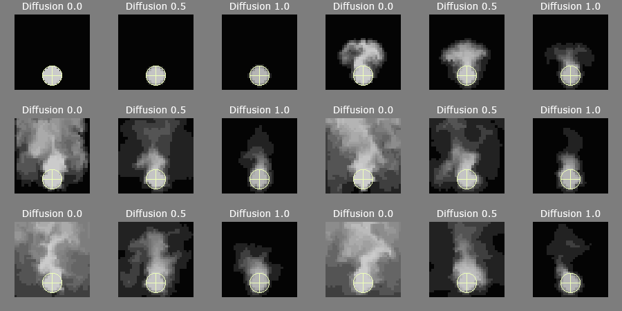
Diffusion: Controls the amount of spread for the density. Higher values intensifies the spread. Setting it to Zero will not spread the smoke.
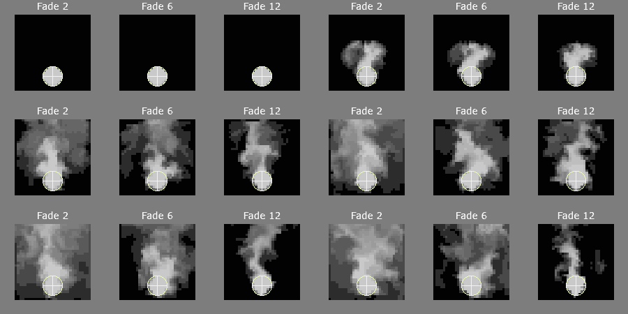
Fade Density: Lessens the density through time. Higher values fades the smoke faster.
Velocity (%): Higher values adds additional velocities which can result to more movement in the grid.  Lower values subtracts velocities, simulating a Drag force.

Bouyancy By: This creates an effect that simulates a smoke rising due to its density.
Density: Moves the velocites upwards due to the density. High density areas will move faster upwards.
Temperature: The solver calculates an average temperature based on the density for whole grid, this setting controls how much of that temperature is used to move the densities upwards.

Extents – Use Boundaries: Enable this to confine the smoke to the Grid boundaries.
Left, Right, Top, Bottom: You may individually control which sides of the Grid are bounded.

---

Set Velocity and Density

Set Velocity

Set Density

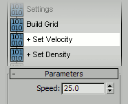
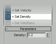
These are Data Icon Operators that can be animated in the viewport to affect the Simulation Grid. It will only affect particle voxels that are inside the Sphere Icon.

Speed: The sphere icon will generate velocities based on its movement, you can set the multiplier value here. Higher speed multiplier generates faster velocities.
Density: Simply sets the density for voxel particles found inside the Sphere Icon.

I also added a special Set Velo/Dens Operator that acts like the Set Density op, but with an added directional speed. The direction is controlled by the icon alignment along its x-axis. The movement of the Data Icon op does not affect the grid though.

---

Start Simulation

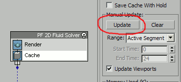
To start the simulation, you may actually just drag the time slider and wait for it to calculate. For low Cell settings like 5-10, the speed is acceptable. But on larger Cell counts like 30+, I recommend using the Cache Operator to simulate the fluid.

Cache – Simulate

---

Parameter Studies

Here are some sample tests on various parameter settings and its effect on the simulation.

Cell Size

Viscosity

Diffusion

Density Fade

Velocity

Bouyancy by Density

Bouyancy by Temperature

Bouyancy by Density and Temperature

Boundaries

Show Velocites

---

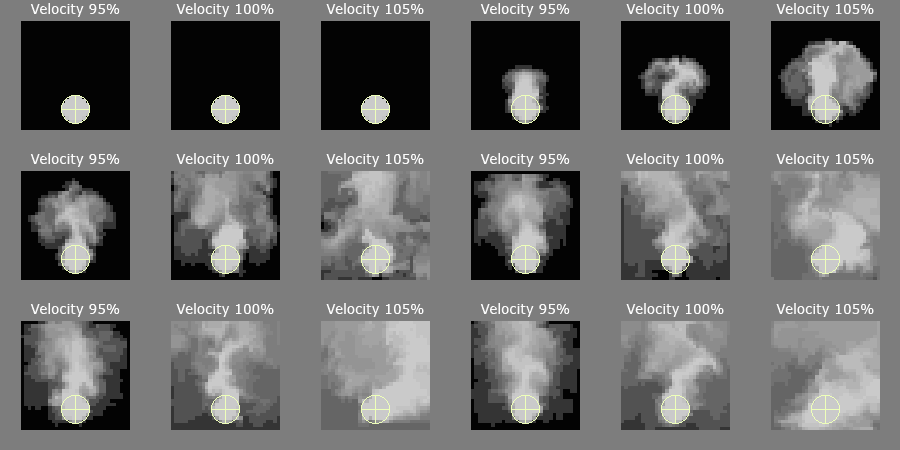
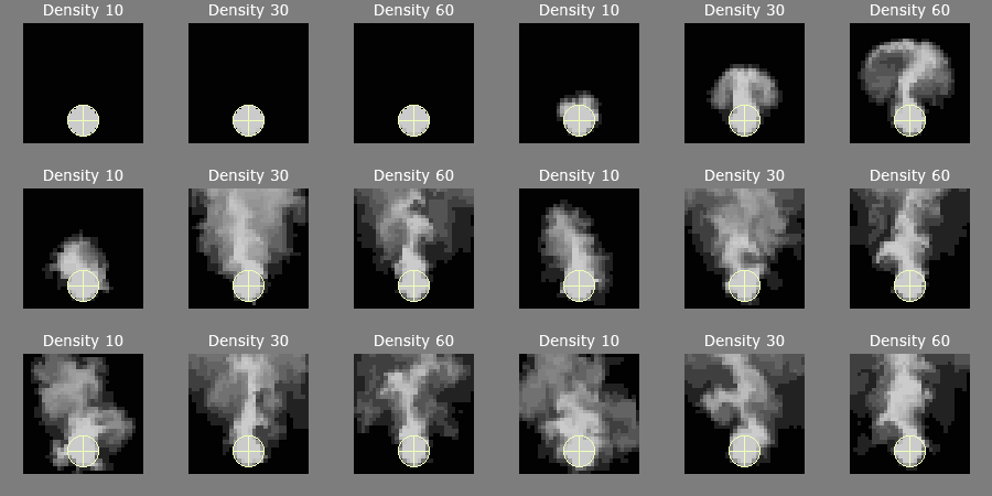
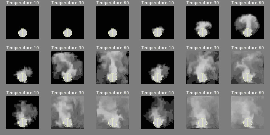
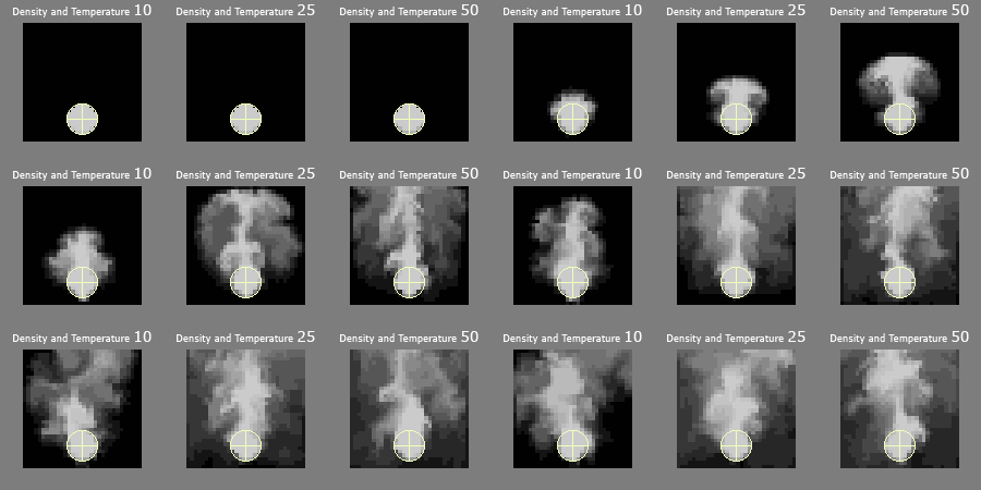
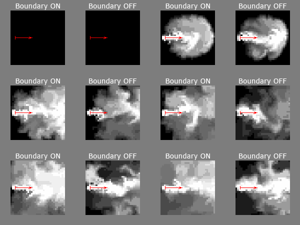
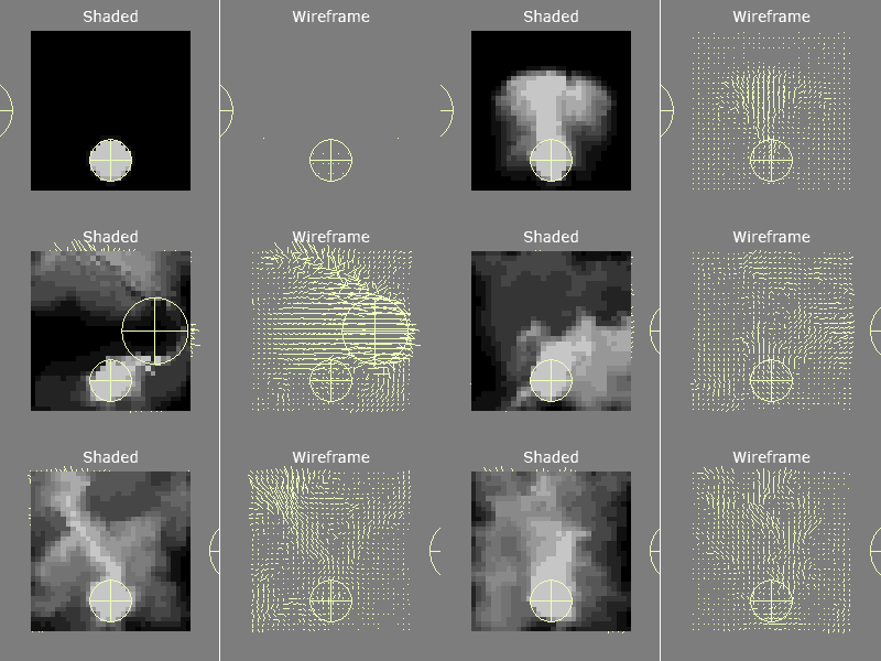
Examples

Here are a few more tests playing with some other possible implementations, all using box#3 operators to extend the system.

1. Gradient Color
I colored the Gradient Ramp to look like fire. This one is actually included in the provided max file at the Orbaz Forums, you just need to replace the material assigned to the particles in the Density Visualization Event with the Flame Material found in the Material Editor.

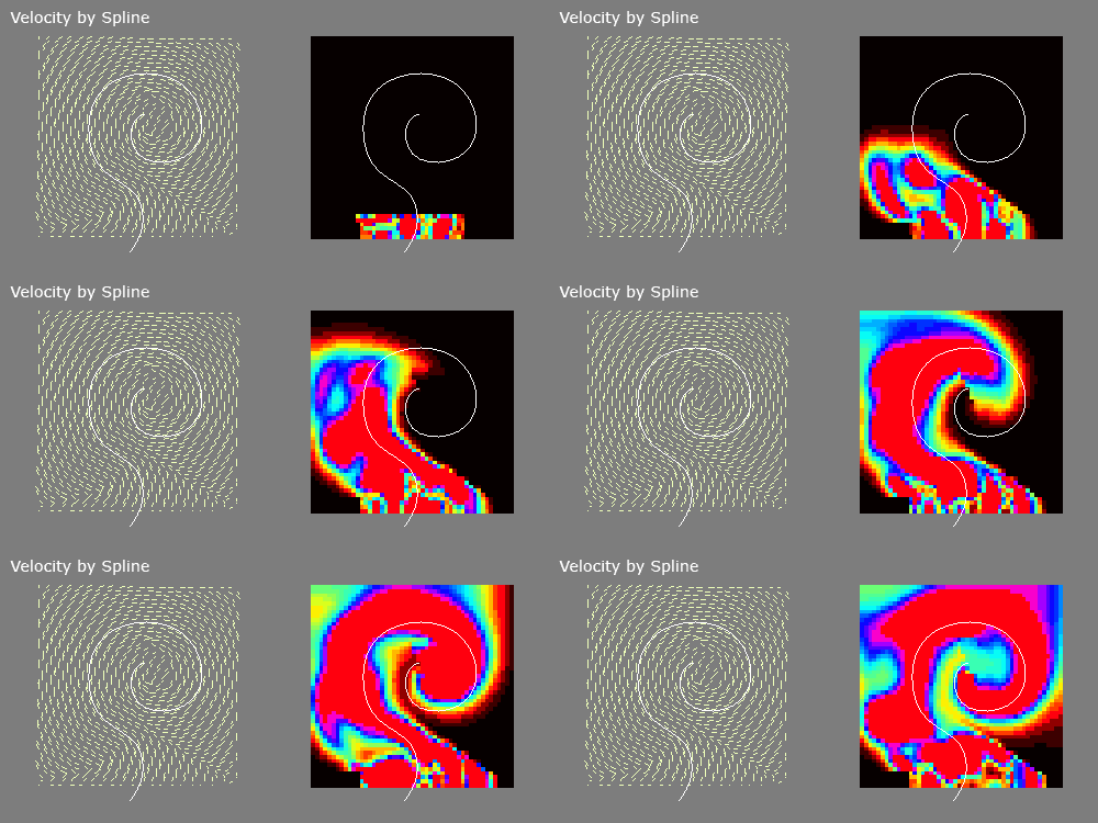
2. Velocity by Spline
This one creates a velocity field based on a spline path. I used a separate particle system to define a vector that goes along the length of the spline. Which is then read by the solver to define the velocities for the sim.

3. Particles as Source
This sample uses a particle system as an emitter of densities and velocities.

4. Re-Using Velocities
These two examples uses the velocities generated by the solver (which is now cached).
Left – Emits particles continuously.
Right – Emits particles only on the first frame.

5. Advecting UVs
I reused the process used by the density solver and passed it UV mapping data for advection.

---

Files:

• 3dsMax 2010 File: PFlow 2D Fluid Solver (Orbaz Forums link)
• MaxScript File: (OK, I decided to add the maxscript as a separate blog entry where I’ll also post a code by code conversion to box#3)

Notes:

• The simulation is very SLOW compared to it’s MaxScript counterpart.
• The system helps in visualizing the operations that are happening inside a fluid solver.
• Notice that I also used multiple copies of some Data Ops like Set Boundary and Advect, this is because the system is currently limited in re-using existing Data flows. If you were to relate this to MaxScript, it’s like the system does not allow you to re-use Functions definitions.
• Higher number of cells tend to loose its swirliness.
• The file also has a plane object lying around, it helps to get a faster response upon loading the scene.
  Try this to see the difference:
  1. Open the 2D Fluid Solver scene file.
  2. Delete the Plane object.
  3. Save the Scene as a different file.
  4. Load the saved file.
     * Notice how the viewport response slows down.
     * A way to fix that is to create any object in the scene — it kinda wakes up the viewport to respond much better.
     * I’m not actually sure if this bug only happens on max2010 though..

To Do:

• Promote it to become a 3D Solver (though it will definitely be a lot MORE slower).
• Add Object Emitters.
• Try out other Iterative solvers (Conjugent?)
• Apply a turbulence field.